The central limit theorem makes averages look normal

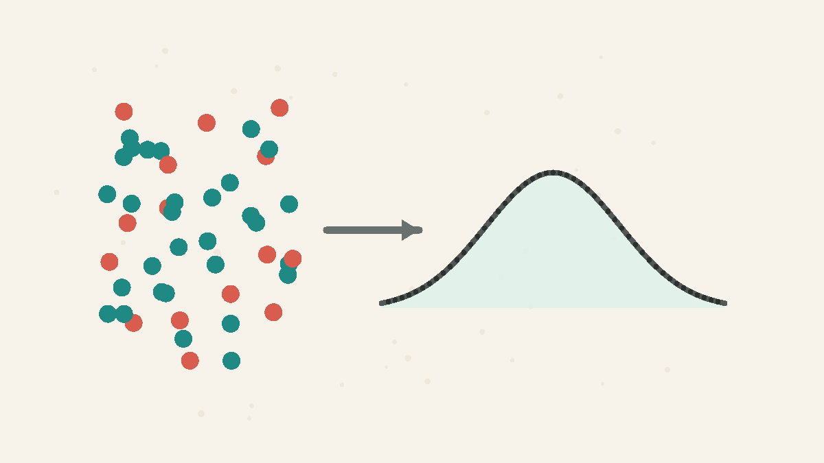
Individual data can be skewed or messy, while averages of many independent observations often form a neat bell-shaped pattern.

The central limit theorem explains why averages are often easier to model than individual observations, even when the raw data are not normally distributed.

By the Math Says Yes editorial team

Human-reviewed under our source and correction standards.

How we review content

THE TRAP

Thinking the theorem says raw data are normal, when it is really about the distribution of repeated averages.

Messy individual dots flowing into a smooth bell curve of averages.

The surprising part

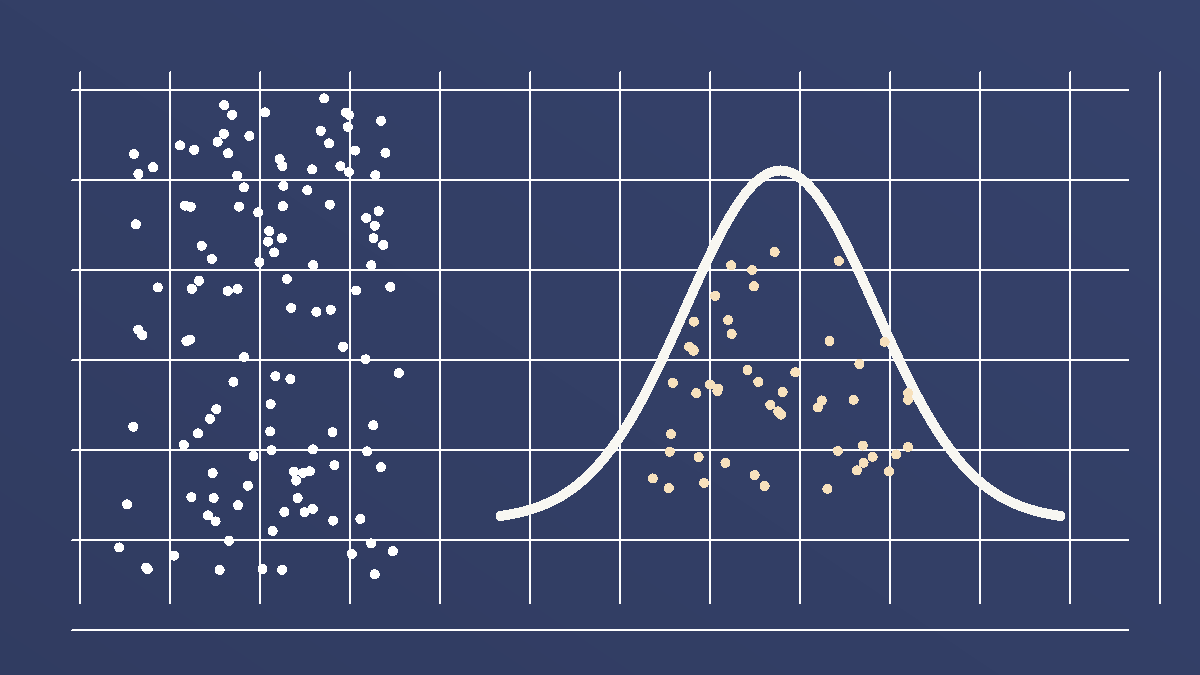
Many real datasets are not bell-shaped. Purchases are skewed, waiting times stretch rightward, and social counts can have long tails. Yet if you repeatedly take samples and each , the of those averages often becomes bell-shaped. The original observations stay messy. The averaging process creates a cleaner sampling pattern.

What the Numbers Show

single purchases

averages of 50 purchases

purchase amount →

Individual purchases are skewed. Repeated averages of 50 purchases form a bell around the mean of about 30.

What the theorem says

enough independent random quantities — dice rolls, measurement errors, daily purchase amounts — and, under broad conditions, the result tends toward a after appropriate scaling. The exact conditions matter, but the intuition is simple: each observation pushes the average a little. When many small independent pushes combine, their total error has a stable shape. That stable shape is why normal-based standard errors and confidence intervals are common.

What it does not say

The theorem does not make every small dataset safe to treat as normal. It does not erase dependence, selection , or one huge observation that dominates the . It also does not say that individual people, purchases, or events are normally distributed. The normal shape belongs to the repeated average under suitable conditions. Confusing those two levels is the common mistake. The theorem explains the average's error, not every observation's shape.

How to use it

Use the when the question is about an or total and the observations are reasonably independent. Check the and whether outliers dominate the result. If the conditions look reasonable, normal-based uncertainty can be a practical approximation. If they do not, simulate the sampling process or use methods designed for skewed, dependent, or heavy-tailed data. The conditions decide whether the shortcut is fair.

Worked example

Daily purchase amounts in a shop might be strongly skewed: many small purchases and a few very large ones. A single purchase is not bell-shaped. But if you repeatedly 50 purchases and each sample, those sample averages can cluster in a much more regular, bell-like way. The theorem is about that repeated-average pattern, not about forcing the raw purchase amounts to look normal.

When it applies

The is a powerful approximation, not a magic spell. It works best when observations are reasonably independent, no single observation dominates the total, and the is large enough for the at hand. Heavy tails, dependence, clustered sampling, and strong selection can slow or break the approximation. In those cases, simulation, resampling, or a model tailored to the data shape may be safer.

What people get wrong

People often turn the theorem into "large samples make data normal" or "n = 30 is always enough." The theorem is narrower and more useful than that. It describes the of sums or averages under conditions. It does not guarantee that raw observations, biased samples, or dependent data behave normally.

Source note

Le Cam's historical account supports the page's framing that the is a family of precise mathematical results with conditions, not a casual rule that all data become normal. The background source supplies the standard statement; the trusted source anchors the caution about interpreting the theorem at the correct level.

FAQ

Does the central limit theorem apply to small samples?

Sometimes, but not automatically. The approximation works better with larger samples and weaker tails, and worse when observations are dependent or dominated by extreme values.

Why does the central limit theorem matter for confidence intervals?

It often justifies using a normal-shaped sampling distribution for an average, which makes standard errors and confidence intervals practical even when the raw observations are not normal.