Fact
Twice as much data does not make estimates twice as precise
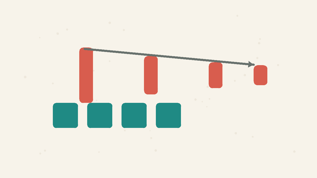
For many averages, cutting random error in half takes about four times as many observations. Precision has square-root returns.
Standard error shrinks with the square root of sample size, which is why small samples wobble and very precise estimates get expensive fast.
By the Math Says Yes editorial team
Human-reviewed under our source and correction standards.
How we review content
THE TRAP
Assuming precision improves in a straight line with sample size, so twice the data should mean half the error.
What standard error measures
is the typical wobble of an estimate across repeated samples. If you repeatedly sampled the same and computed the each time, those means would not be identical. They would form their own around the true mean. The standard error describes the spread of that distribution, so it tells you how much random sampling noise remains in the estimate.
What the Numbers Show
10
100 readings
7.1
200 readings
5
400 readings
With 100 readings the typical wobble is ±10 points; 200 cuts it to about ±7, and 400 reaches ±5.
The square-root catch
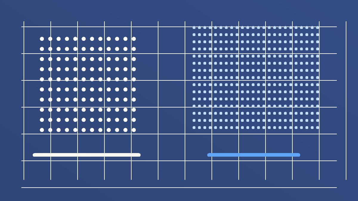
Moving from 100 to 400 observations cuts the error about in half; moving from 400 to 1,600 cuts it in half again. The shrinks like one divided by the square root of n. That is good news because more data helps. It is also humbling because the improvement slows down: the same precision gain gets more expensive each time.
Why intuition fails
Most everyday quantities feel linear: twice the money buys twice the item, twice the distance takes twice the time, and twice the workers can sometimes do twice the work. Sampling precision is different because random errors cancel in both directions. More observations add information, but they also add new random variation. The averaging process wins gradually, and the square-root rule is the pace at which it wins.
How to use it
When someone asks for a much tighter estimate, translate that request into . Half the random error usually means four times the ; one-tenth the error means about one hundred times the sample. This does not more data is pointless. It means precision has a price, and good study design should decide whether that price is worth paying for the decision at hand.
Worked example
With 100 observations, you divide the raw scatter by 10, the square root of 100. That is the whole recipe: if the of individual measurements is fixed, the of a is that standard deviation divided by the square root of the . With 400 observations, the divisor is 20, so the standard error is cut in half. Doubling from 100 to 200 only changes the divisor from 10 to about 14.1, which is a useful gain but not a two-times precision gain.
When it applies
The square-root rule describes random sampling noise under assumptions such as independent observations and a stable . It does not that any larger dataset is automatically better. If the new data come from the wrong population, repeat the same measurement error, or are selected in a biased way, the can look smaller while the estimate remains wrong.
What people get wrong
Twice the survey budget, twice the records, or twice the experiment time feels like it should halve the uncertainty. Random does not work that way, and precision does not scale like effort. The square-root relationship means precision improves, but the easy gains arrive early.
Source note
Altman and Bland explain the difference between and , including why standard error measures precision of an estimate rather than variability among individuals. That distinction is the basis for the page's main lesson: increasing improves precision through the sampling , but the improvement follows a square-root curve.
FAQ
Why does standard error shrink with the square root of sample size?
Independent random errors partly cancel when averaged. The math of variance makes the spread of the sample mean shrink with the square root of n, not directly with n.
Does more data always solve uncertainty?
More representative data reduces random sampling error, but it does not fix bias, bad measurement, nonresponse, confounding, or a sample that misses the population you care about.
Quick Check
If you want to cut the standard error of an average in half, roughly how much more data do you need?
A
About twice as much data.
B
About four times as much data.
C
About half as much data.
Sources
Standard deviations and standard errors
Primary source
BMJ · Accessed 2026-06-20
Standard error
Secondary explainer
Wikipedia · Accessed 2026-06-16
Know someone who'd like this?
Read next
The smallest towns top both the best and worst lists
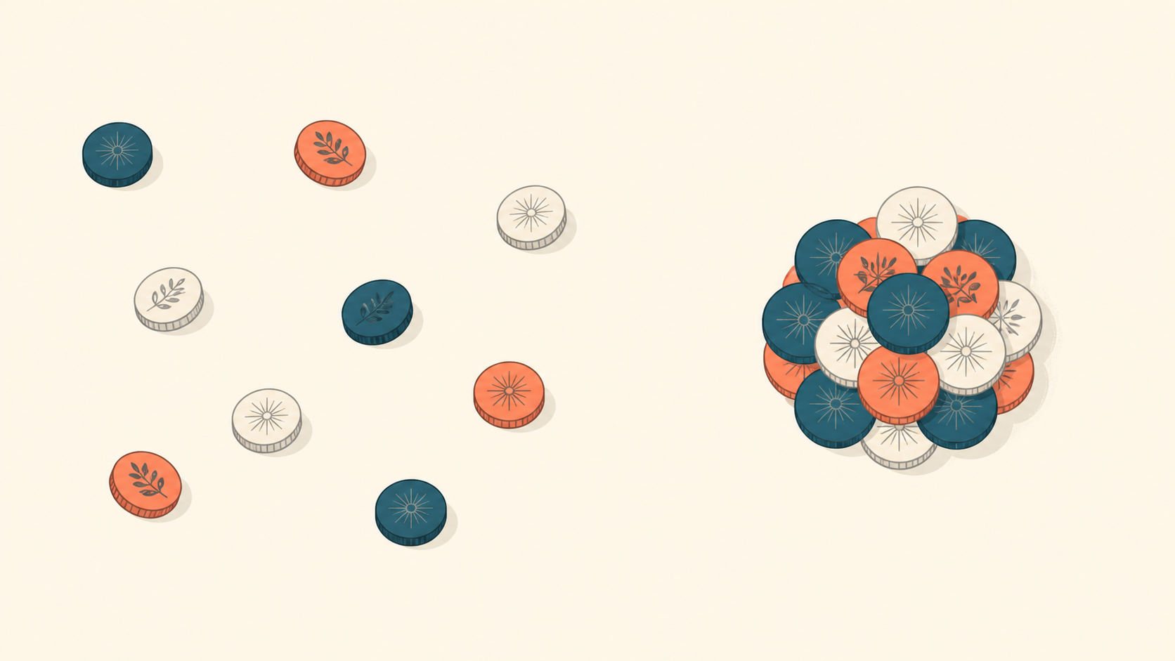
Rank places by any rate — cancer, test scores, crime — and the extremes are dominated by the smallest places, because small samples swing far from the true rate by luck alone.
Concepts
Law of Large Numbers
As a sample grows, its average gets closer to the true average and random swings shrink, roughly in proportion to 1 over the square root of the sample size. Small samples can land far from the truth purely by chance, which is why a handful of observations is so easy to misread.
Standard Error
Standard error is the typical sampling wobble of an estimate such as a mean. For independent observations, the standard error of a mean shrinks with the square root of the sample size, so cutting the error in half usually takes four times as much data.